TL;DR of the paper 'Cube-to-sphere projections for procedural texturing and beyond'

I will in this post write down a TL;DR of the paper 'Cube-to-sphere projections for procedural texturing and beyond'. Observe that all images are from the paper, and do not belong to me

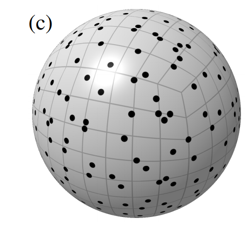
For drawing a procedural texture on a sphere, we basically need to place out a bunch of sample points on a sphere, as is illustrated in the image.

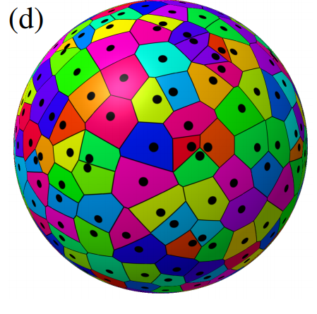
For voronoi noise, we need to place out jittered sample points on a sphere. That is, sample points that don't clump together. Then, we can produce the texture below as follows: assign a random color to each sample point. The color of every point on the sphere, is just the color of the nearest sample point

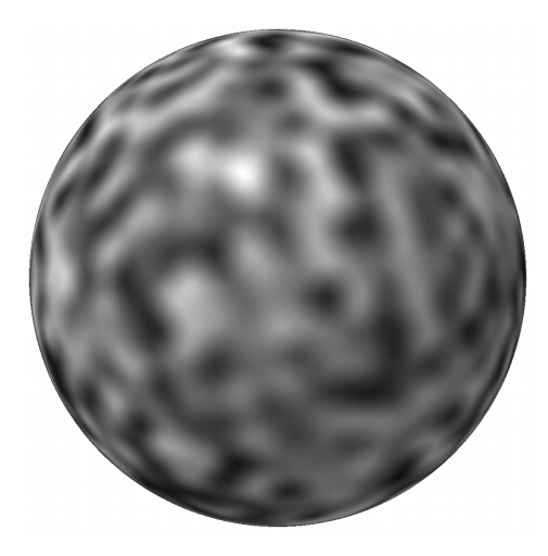
On the other hand, for value noise, we need to place out sample points that are equally distant from each other. We then make value noise as follows: assign a value to each sample point, and interpolate between the 4-nearest sample point values, to get the color of a point on the sphere.

As we can see from the above, for both value noise and voronoi noise, we need a way of finding the $k$-nearest sample points. This is IMO the main theme of the paper.

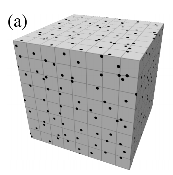
Their method is pretty simple: they take a cube, and subdivide each face into cells. Place exactly one sample point at a random position in each cell, and we get a nice jittered sampling, usable for voronoi noise.

And place one sample point in the center of each cell, and we get a sampling usable for value noise.

Now, we simply project this cube onto a sphere. That is, we apply some function that makes this cube into a sphere. In the end, this means that every sample point is projected onto some corresponding position on the sphere.

Now this function should be as area preserving as possible. That is, a small area on the cube, should be transformed into a small area on the sphere. This makes sure that the nice properties of our sampling is preserved. So that if the sample points have a jittered distribution, then they will keep their jittered distribution, even when projected onto the sphere.

Now, we also want this function to be invertible. Because then, we can recover the original grid cell of the point(before the projection) by simply using this inverse function.

So, given some point on the sphere, we find the closest $k$ sample points as follows: apply the inverse function to that point. It will then be projected to one of the faces of the cube, and we can recover the exact grid cell easily, because the point will be projected into one of the grid-cells of the face(study the image below). Finally, we can now find the closest $k$ sample points by looking in the surrounding grid cells, and finding the $k$ ones that are closest. This is much faster than looking through ALL the sample points.

The authors examine several functions for performing the projection from the cube to the sphere. The simplest approach for projecting some position $p$ on the cube to the sphere, is that you simply normalize $p$. But this has a relatively high amount of area distortion.

The authors examines a different approach: every point on the cube will fall into one of the six faces. A point within the face can be determined by two coordinate values, and they apply a function to both these two values, that warps them. After warping the point, they normalize the point, to complete the projection. The point of the warping is to make it more area preserving.

For instance, in one particularly successful warp function, the values are warped by a fifth-order polynomial. They find the coefficients of the polynomial by running an optimization that minimizes the amount of area distortion. In order to approximately invert the polynomial, they, again, do an optimization to find a polynomial that approximates the inverse.