An Intuitive Explanation of using Poisson Blending for Seamless Copy-and-Paste of Images

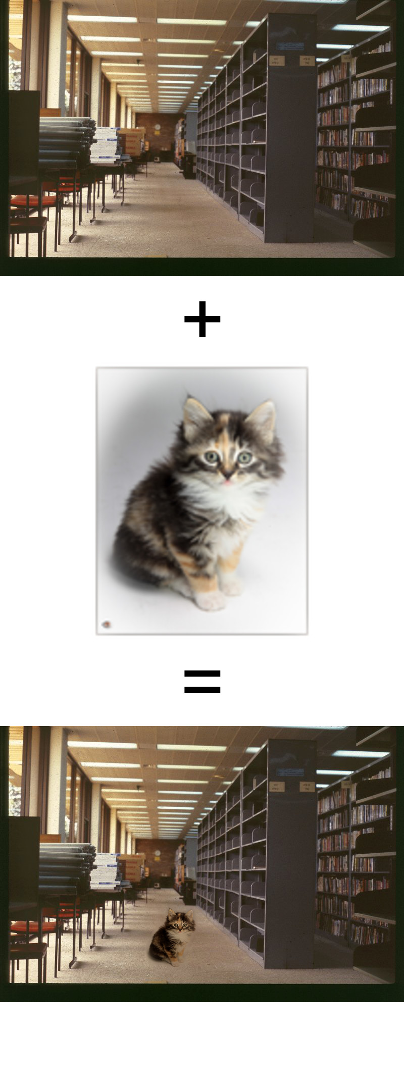
$\newcommand{\mvec}[1]{\mathbf{#1}}\newcommand{\gvec}[1]{\boldsymbol{#1}}\definecolor{eqcol2}{RGB}{114,0,172}\definecolor{eqcol1}{RGB}{172,0,114}\definecolor{eqcol3}{RGB}{0,172,114}\definecolor{eqcol4}{RGB}{230,190,120}$In this article, we explain the intuition behind an image processing technique called Poisson Blending. This technique is an image processing operator that allows the user to insert one image into another, without introducing any visually unappealing seams. Furthermore, this technique also makes sure that the color of the inserted image is also shifted, so that the inserted object feels as if it is part of the environment of the target image. So a bright object copy-and-pasted into a rather dark image, will have its color shifted to a darker color. In the below image, an image of a kitten has been copy-and-pasted into an image of a library using poisson blending, and as can be observed, there are no visible seams.

This article explains how to implement the concepts first described in Section 2 and 3 of [1].

Image Gradients as an Image Encoding Scheme

Before we can explain poisson blending, a more fundamental concept must first be clarified to the reader: image gradients. In the following explanation, a one-dimensional grayscale image will be used for explanations, in order to simplify the mathematical expressions. Consider the following bar chart

The bar chart represents a grayscale image, where the first pixel has a grayscale value of $f_1 = 6$, the second one $f_2=4$, and so on. As can be observed, the image has a pixel width of 8, and it is visualized as a grayscale image below

One approach to encoding this image is by simply saving the grayscale values of every pixel, $f_1, f_2,\dots f_8$. However, an alternative way of representing them, is to instead store the gradients of every pixel. In one dimension, the gradient is simply the derivative. As an example, the derivative in the positive $x$-direction at $f_3$ can be found from the definition of the derivative \[ \frac{f_{3 + \Delta x} - f_{3}}{\Delta x} = f_{4} - f_{3} = 2 \] Where we have let the step-size be $\Delta x = 1$. This is how the gradient of a pixel in an image is defined. We denote the above derivative as $v_{4,3}$, and in general, we define the gradient between the pixels $p$ and $q$ as $v_{p, q} = f_p - f_q$. This value is simply the change in grayscale intensity, as we go from $q$ to $p$. Something that is remarkable, is that we simply need to store all gradients, and some boundary conditions in order to encode the entire image.

We now demonstrate how the pixels represented by the yellow bars can be encoded(we shall deal with the gradients in both the positive and negative directions, and we do this to keep our notation consistent with the one used by [1]. It is actually only necessary to store the positive gradients). Their gradients are $v_{2,3} = 1$, $v_{3,2} = -1$, $v_{3,4} = -2$, $v_{4,3} = 2$, $v_{4,5} = 1$, $v_{5,4} = -1$, $v_{5,6} = -2$, $v_{6,5} = 2$, $v_{6,7} = -2$, and $v_{7,6} = 2$. Given only these values, it is not possible to restore the values of the yellow bars. However, if we also have the boundary conditions $f_2 = 4$ and $f_7 = 8$(which we hereon denote as boundary conditions), then it becomes possible to recover the values of $f_3$, $f_4$, $f_5$ and $f_6$. Because since we know that $v_{3,2} = f_3 - f_2 = -1$, and given our boundary condition $f_2 = 4$, we can solve for $f_3$: \[ f_3 = v_{3,2} + f_2 = -1 + 4 = 3 \] Following this, we can easily solve for $f_4$, using our given value for $v_{4,3}$, and so on. To conclude, given the boundary conditions, and the values of the gradients, we can always recover the original image.

We have just recovered the original image though hand calculation, but we of course also need to construct an algorithm that we can describe to the computer. We will recover the image by formulating an optimization problem, and solving it. For the pixels $f_3$ and $f_4$, the difference between them should be as close as possible to $v_{4,3}$. This means that the quantity $(f_4 - f_3 - v_{4,3})^2$ should be as small as possible(we square it to remove any negative values. We are merely interested in how close this value is to zero, not its sign). The same statement should be true for all the adjacent pixel pairs, and all these pairs will have such a squared difference term associated with them. Summing all these terms up, we obtain the energy function $h$ \begin{align*} h(f_3, f_4, f_5, f_6)& =\\ &(f_3 - f_2 - v_{3,2})^2 + (f_2 - f_3 - v_{2,3})^2 \\ &(f_4 - f_3 - v_{4,3})^2 + (f_3 - f_4 - v_{3,4})^2 \\ &(f_5 - f_4 - v_{5,4})^2 + (f_4 - f_5 - v_{4,5})^2 \\ &(f_6 - f_5 - v_{6,5})^2 + (f_5 - f_6 - v_{5,6})^2 \\ &(f_7 - f_6 - v_{7,6})^2 + (f_6 - f_7 - v_{6,7})^2 \\ \end{align*} By minimizing this function, we will find the values of $f_3$, $f_4$, $f_5$ and $f_6$ that as close as possible preserve the values of the given gradients. By finding these values, we will have recovered the original image from the gradients. Observe that $h$ is quadratic in terms of its variables $f_3$, $f_4$, $f_5$ and $f_6$, so minimization can be done by finding the partial derivatives with respect to all these variables, and then finding the point at which all these partial derivatives are zero. As an example, we take the partial derivative with respect to $f_5$. \begin{align*} \frac{\partial h}{\partial f_5} &= 0 \\ 2(f_5 - f_4 - v_{5,4})- 2(f_4 - f_5 - v_{4,5}) - 2(f_6 - f_5- v_{6,5}) + 2(f_5 -f_6 - v_{5,6}) &= 0\\ \end{align*} since $v_{p,q} = -v_{q,p}$ simplification gives us \begin{align} 2f_5 - f_4 - f_6 &= v_{5,4} + v_{5,6} = -3 \label{eq:partialderiv} \end{align} The gradients, which are already known, are on the right side, and on the left-hand-side we can find our unknown variables, $f_5$, $f_4$ and $f_6$. We will obtain a similar result when computing the partial derivative with respect to $f_4$. For $f_3$ and $f_6$, the result is different, since the boundary conditions must be taken into account. For $f_3$, we find that \begin{align*} 2f_3 - f_4 &= v_{3,2} + v_{3,4} + f_2 = 1 \end{align*} since $f_2$ is a boundary condition and therefore its value is known, it ends up on the right side.

To summarize, if we take the partial derivative of our energy function $h$ with respect to all the variables, and set them to zero, we obtain the system of linear equations. \begin{align*} 2f_3 - f_4 &= 1 \\ -f_3 + 2f_4 - f_5 &= 3 \\ -f_4 + 2f_5 - f_6 &= -3 \\ -f_5 + 2f_6 &= 8 \\ \end{align*} We write this system in terms of matrices, \begin{equation*} \begin{bmatrix} 2 & -1 & 0 & 0 \\ -1 & 2 & -1 & 0 \\ 0 & -1 & 2 & -1 \\ 0 & 0 & -1 & 2 \\ \end{bmatrix} \begin{bmatrix} f_3 \\ f_4 \\ f_5 \\ f_6 \\ \end{bmatrix} = \begin{bmatrix} 1 \\ 3 \\ -3 \\ 8 \\ \end{bmatrix} \end{equation*} To recover the original image, we simply give this linear system to a linear solver(in our code, we used Eigen and a Cholesky Decomposition for solving), and it will give us back the original image. This can easily be verified by Wolfram Alpha.

Poisson Blending

We have shown that the original image can be reconstructed from the gradients and a number of boundary conditions. We will next demonstrate how this fact can be used to seamlessly copy and paste one image into another. First, let us say that we have the below source image.

which can be represented by the bar chart

We wish to paste the pixels $f_3$, $f_4$, $f_5$ and $f_6$ into the corresponding pixels in the target image, which is the image we dealt with in the precision section. However, just copying and pasting those pixel values does not give good results:

The bar chart of the above image allows us to visualize why

The source image has much brighter values than the target image. If the pixel values from the source image are just copied and pasted, this will result in a harsh and sudden change of color, from the pixel $f_2$ to $f_3$. In a two-dimensional image, the result is even more unappealing, which can be seen in the images in the next section.

The values of the source image must be modified, in order to make the transition less harsh. To be more specific, some form of blending must be performed between the source and the target image. The idea behind poisson blending is simple: we encode the target image as gradients, but at the area into which we wish to copy and paste the source image, we simply copy and paste the gradients of the source image. That is, in the area of copy-and-paste, the original gradients are replaced with the source gradients, and we then simply recover an image from these modified gradients, just like we did in the previous section. In the previous section, we took the partial derivative with respect to $f_5$ and obtained equation $\eqref{eq:partialderiv}$. However, if we are using poisson blending, the gradients on the right side will have different values. The gradients will instead be calculated from the source image, so that the expression becomes \begin{align} 2f_5 - f_4 - f_6 &= v_{5,4} + v_{5,6} = (g_5 - g_4) + (g_5 - g_6)= 4 + 5 = 9 \end{align} The right hand side assumes a different value, since our gradients have been modified. This occurs for all the other three equations in the linear system, and the modified linear system becomes \begin{equation*} \begin{bmatrix} 2 & -1 & 0 & 0 \\ -1 & 2 & -1 & 0 \\ 0 & -1 & 2 & -1 \\ 0 & 0 & -1 & 2 \\ \end{bmatrix} \begin{bmatrix} f_3 \\ f_4 \\ f_5 \\ f_6 \\ \end{bmatrix} = \begin{bmatrix} 10 \\ -8 \\ 9 \\ 1 \\ \end{bmatrix} \end{equation*} Note that we have used the boundary conditions from the target image, so that $f_2 = 4$ and $f_7 = 8$. Solving this system, we obtain the poisson blended image seen below.

Which can be visualized as

The intensity of the grayscale values in the source image has been shifted down, so that they have about the same intensity as the target image. This is thanks to the boundary conditions $f_2 = 4$, and $f_7 = 8$, which were from our original target image. The linear system comes from an optimization problem, and this optimization problem ensures that the gradient of $v_{3,2}$ of our recovered image is as close as possible to the value $26 - 24 = 2$(gradient of the source image). In our recovered image, that gradient assumes the value $7 - 4 = 3$. It would have been very unlikely that the recovered image would have assumed the value $26$ at $f_3$(as in the original source image), because then the gradient would be $26 - 4 = 22$ in the recovered image, which is a rather large value, which exactly the situation the solver is strifing to avoid.

Another thing that we wish to remark is that even though poisson blending shifts the color of the source image, it still preserves the features of it. In the original source image, $f_4$ is smaller than $f_3$, $f_5$ is greater than $f_4$, and so on, and this also applies to our recovered image. This information was encoded by the gradients of the source image. However, it is also important to realize that poisson blending does not exactly preserve the gradients. In the recovered image, the gradient $f_{3,4}$ assumes the value $7 - 4 = 3$, but it was $26 - 22 = 4$ in the original source image. In the previous section, the gradients of the recovered image were identical to the gradients of the original image. But with poisson blending, the gradients of a completely different image are pasted into another image, and the result of this is that the solver is not always able to recover an image whose gradients exactly match the specified gradients. But the solver tries to find an image whose gradients match as close as possible, and in practice, poisson blending yields good results, which we shall show examples of in the following section.

Two-Dimensional Poisson Blending

In the previous section, the intuition behind poisson blending was described for one dimension. Everything in the previous section generalizes readily to a two-dimensional image. In the one-dimensional case, there was only a derivative in the $x$-direction, but for two dimensions, we must also take into account the derivative in the $y$-direction. However, this fact introduces little additional complexity, and formulating and minimizing an energy function is just as straightforward as in one dimension. In the interest of brevity, we will provide no further details in the article. We provide code that demonstrates how to implement poisson blending in two dimensions, and the reader is encouraged to study this code(and the reader is also referred to equation (6) of [1]. This is the energy function for the two-dimensional case. And (7) represents the resulting linear system that must be solved to minimize this energy function. The provided code demonstrates how to convert these equations to code)

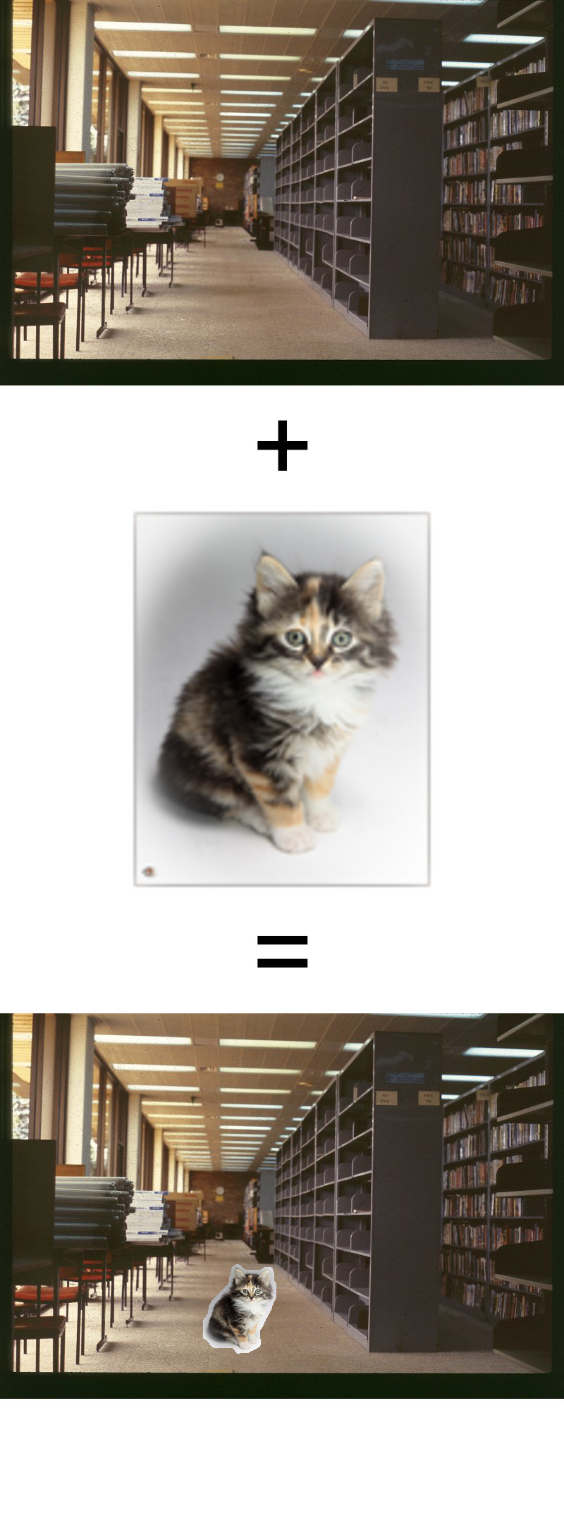
We shall now show some results from the technique. In our test image, we copy and paste a kitten into a library scene. Performing a naive copy and paste gives far from acceptable results.

Naive copy and results in a starkly visible seam. However, using poisson blending instead completely removes this seam:

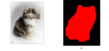
It can also be seen that the color of the kitten has been shifted. The color shift comes from the colors of the boundary conditions, which is the floor in this case. Note that we specify a mask for the kitten image, which is illustrated to the right below

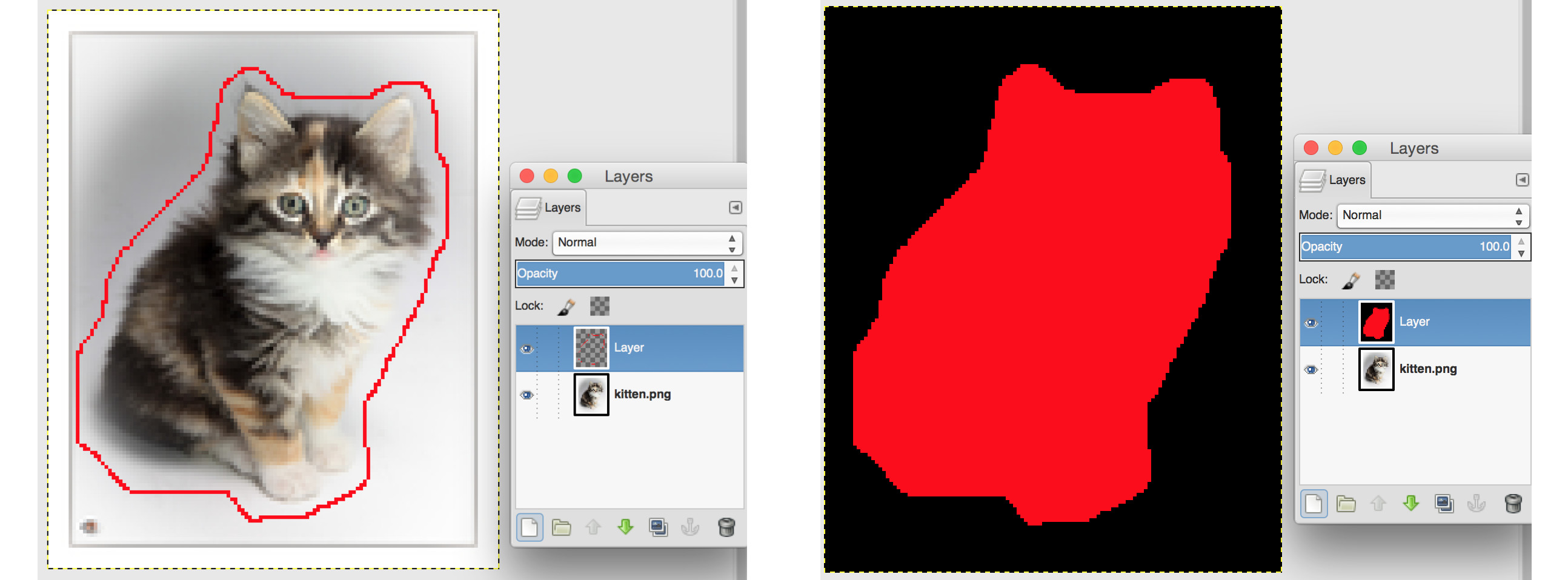
We only perform the poisson blending calculations for pixels within this red area. This allows us to save much performance, since every extra pixel results in an unknown variable in our linear system. Many unknown variables result in a huge matrix equation that needs to be solved, and solving huge matrix equations requires a large amount of calculations and takes time. Such a mask image is easy to construct using an external image editor such as Photoshop or Gimp. In our case, we utilized Gimp to draw a closed loop around the kitten in a separate layer, and then finished the mask by performing a simple flood fill, as is illustrated below.

Finally, the boundary conditions in two dimensions, are the pixels on the border of this red region.

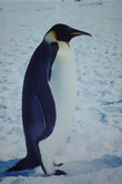
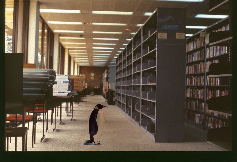
To conclude the article, we will give an example where poisson blending does not give very good results. If we poisson blend the below penguin

Into the library scene, then the result is as follows

The snow background around the penguin can vaguely be seen in the modified library image. Poisson blending has merely modified the color of the snow, but the appearence of the snow is still the same. If the target and source images have very different backgrounds, then poisson blending tends to give not very good results. The kitten image had good results, since it has such a simple background.

This is the end of the article. In a github repository, we provide a commented implementation of poisson blending, and also showcase some more images made using the technique.

References

[1] Patrick Perez, Michel Gangnet, Andrew Blake, "Poisson Image Editing". Link.